ENV221 NOTE

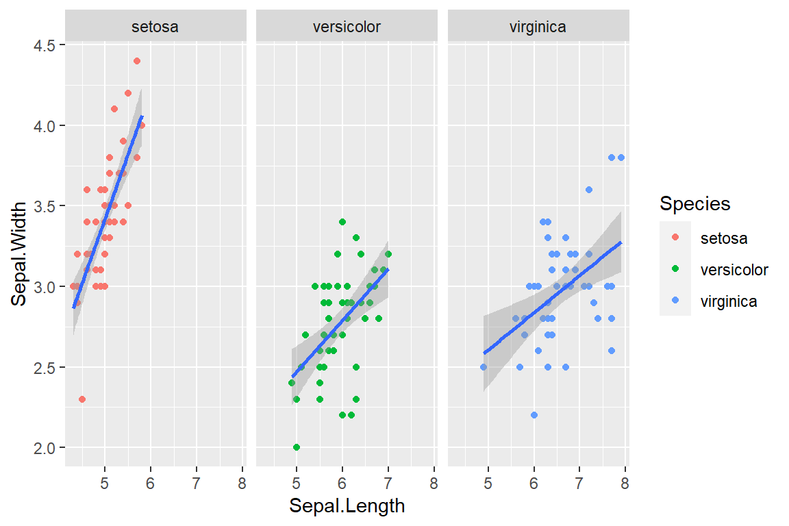
R in statistics (Fundamental)

🚀

Hyperlink of XJTLU ENV221 courseware

• Module overview mindmap
  
• Lecture1 overview
  
• Lecture2 r-basic
  
• Lecture3 r-programming
  
• Lecture4 statistical-graphs
  
• Lecture5 basic-concepts
  
• Lecture6 descriptive-statistics
  
• Lecture7 distributions-and-clt
  
• Lecture8 hypothesis-test
  
• Lecture9 t-test
  
• Lecture10 numerical-vs-numerical
  
• Lecture11 numerical-vs-categorical
  
• Lecture12 categorical-vs-categorical
  

👉🏻Click to enter the ENV222 note section

1 graph part & R basic code

1.1 Scatterplot

library(ggplot2)
ggplot(iris, aes(x = Sepal.Length, y = Sepal.Width)) + 
  geom_point(aes(x = Sepal.Length, y = Sepal.Width, color = Species)) + 
  geom_smooth(method = "lm") + facet_wrap(~ Species)

1.2 Barplot

library(ggplot2)
ggplot(iris) + geom_bar(aes(Species), width = 0.5) + coord_flip()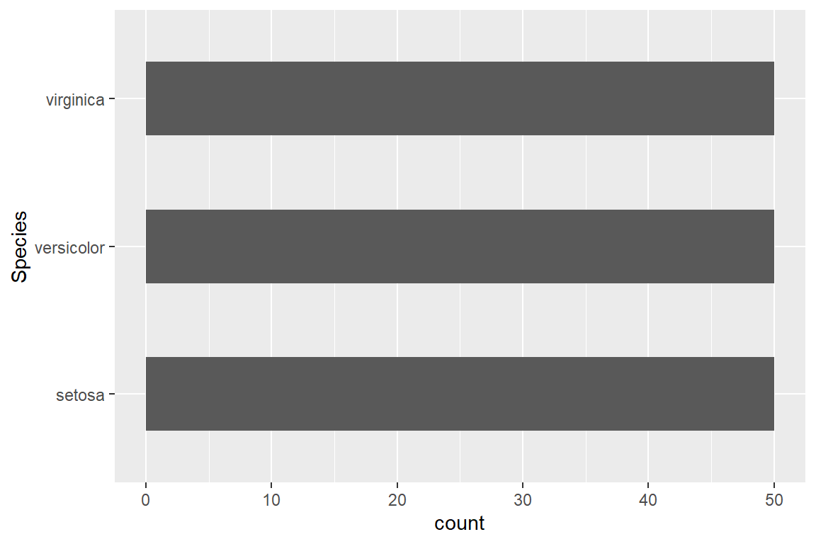

1.3 Histogram

library(ggplot2)
ggplot(iris) + geom_histogram(aes(Sepal.Length))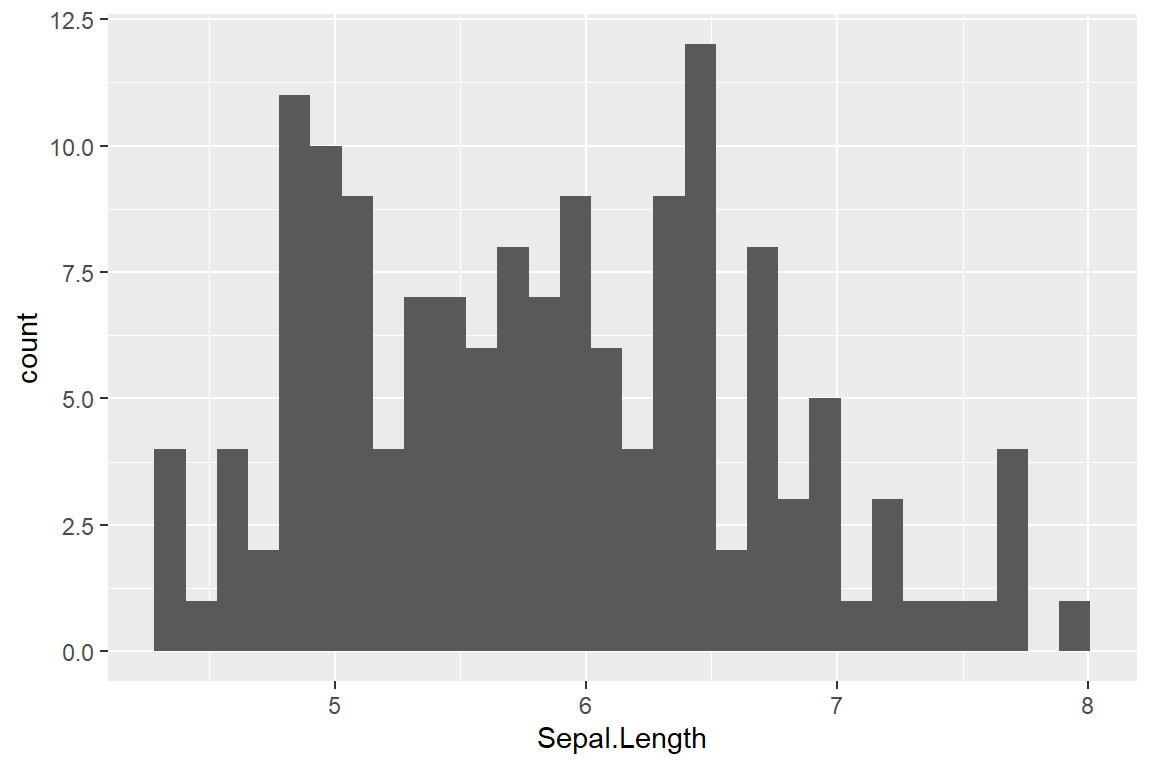

1.4 Boxplot

# R built-in way
River_A <- c(2, 1.95, 1.99, 2.08, 1.99, 1.95, 2.03, 2.09, 2.07, 2.01)
River_B <- c(1.85, 1.94, 1.87, 1.89, 1.91, 1.93, 2.01, 2, 1.96, 1.98)
boxplot(River_A, River_B, names = c('River A','River B'))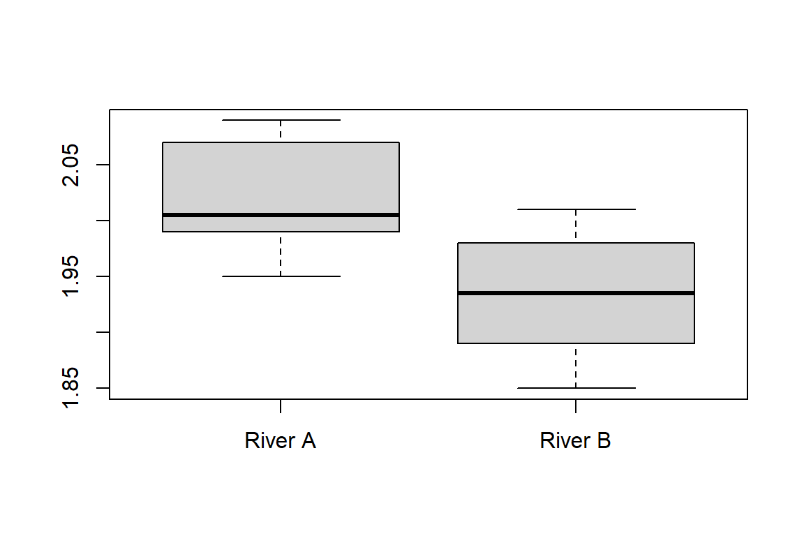

# ggplot2 way
library(ggplot2)
ggplot(iris) + geom_boxplot(aes(Sepal.Length))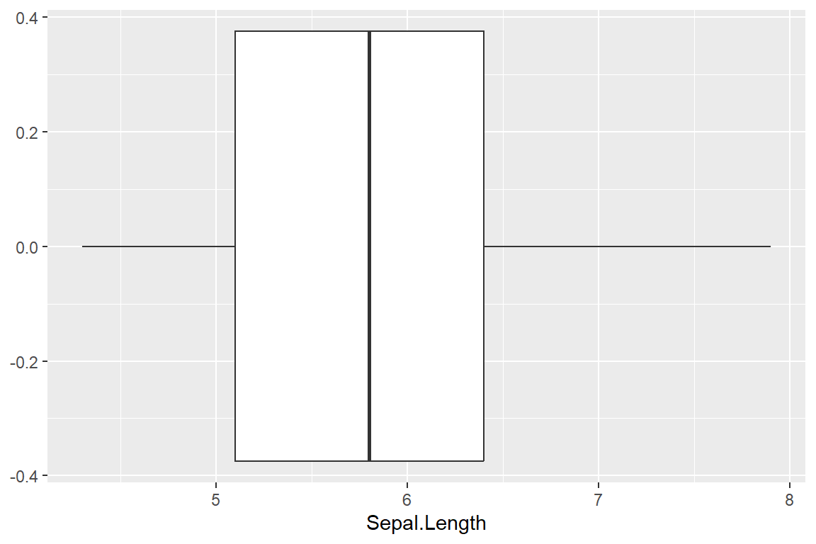

1.5 Pairplot

# install.packages("GGally")
library(GGally)
ggpairs(iris, aes(colour=Species, alpha=0.5))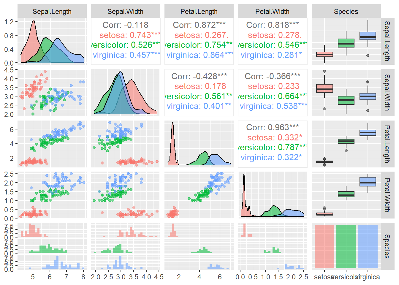

ggsave("df_plot.pdf")   # Save graphs

1.6 R basic operations

# Random sampling
df <- data.frame(x = c(1, 2, 3, 4, 5, 6, 7, 8, 9, 10),
                 y = c('a', 'b', 'c', 'd', 'e', 'f', 'g', 'h', 'i' ,'j'))   
sample(df$y[df$x > 5], 2)

[1] "g" "i"

sample(df$y[df$x <= 5], 2)

[1] "e" "a"

1.7 Two ways to remove NA & outlier from data set

x=c(1,2,NA,4)
mean(x, na.rm = TRUE)   # Remove NA within a function

[1] 2.333333

x <- x[!is.na(x)]   # Adjust dataset (multidimensional data filtering) selected an undefined column. Need to add ', !is.na(***)' after it.
x <- x[x != boxplot(x, plot=FALSE)$out]   # Excluded outliers from the dataset

1.8 Correlation coefficient function

cor_coe <- function(x, y){
  N <- length(x)
  co <- 1 / (N - 1) * sum((y - mean(y)) * (x - mean(x)))
  sx <- sd(x)
  sy <- sd(y)
  co / (sx * sy)
}

2 Statistic part

• H0：Usually, the researcher wants to collect evidence to oppose one side, also known as the null hypothesis (generally including equal to.
• H1：Usually, it is the side that researchers collect evidence to support, also known as the alternative hypothesis (generally including not equal to).
• Type 1 error: False positive (the hypothesis is right but we reject it) [alpha]
• Type 2 error: False negative (the hypothesis is wrong but we didn’t reject it) [beta]
• Alpha(Significance level): The maximum allowable probability of making a type I error [0.10, 0.05, 0.01 …]
• Beta: …
• P-value(Probability value): if P-value <= alpha, reject H0; if P-value > alpha, not reject H0.
• Rejection region, critical region: the range of values for which H0 is not probable(The interval where H0 cannot occur.)

2.1 Binomial distribution

e.g. Toss a coin for “n” times, “x” is the frequency of head

x <- 2
n <- 2
p <- 0.5
dbinom(x, size = n, prob = p)  # Same as choose(n, x) * p^x * (1-p)^(n-x)

[1] 0.25

2.2 Z-test

Known population mean and population variance

x <- c(24, 36, 44, 35, 44, 34, 29, 40, 39, 43, 41, 32, 33, 29, 29, 43, 25, 39, 25, 42, 
       29, 22, 22, 25, 14, 15, 14, 29, 25, 27, 22, 24, 18, 17)
mu <- 29
sd_p <- 9
x_bar <- mean(x)
se <- sd_p / sqrt(length(x))
(z_score <- (x_bar - mu) / se)

[1] 0.4382742

(z_critical <- qnorm(1 - 0.05))

[1] 1.644854

(p_value <- pnorm(z_score))

[1] 0.6694062

2.3 T-test

Known population mean but unknown population variance

mu <- 100
x <- c(91, 100, 70, 87, 104, 92, 104, 88, 72, 119)
t.test(x, mu = mu , alternative = "less", conf.level = 0.05)   # One-tailed

    One Sample t-test

data:  x
t = -1.5478, df = 9, p-value = 0.07804
alternative hypothesis: true mean is less than 100
5 percent confidence interval:
     -Inf 84.05409
sample estimates:
mean of x 
     92.7 

mu <- 0.02
x <- c(0.011, 0.021, 0.001, 0.007, 0.031, 0.023, 0.026, 0.019)
t.test(x, mu = 0.02, alternative = "two.sided", conf.level = 0.1)   # Two-tailed

    One Sample t-test

data:  x
t = -0.73012, df = 7, p-value = 0.489
alternative hypothesis: true mean is not equal to 0.02
10 percent confidence interval:
 0.01690656 0.01784344
sample estimates:
mean of x 
 0.017375 

x1 <- c(24.58, 22.09, 23.70, 18.89, 22.02, 28.71, 24.44, 20.91, 23.83, 20.83)
x2 <- c(21.61, 19.06, 20.72, 15.77, 19, 25.88, 21.48, 17.85, 20.86, 17.77)
t.test(x1, x2, var.equal = TRUE, alternative = "two.sided", mu = 0)   # Two samples

    Two Sample t-test

data:  x1 and x2
t = 2.4396, df = 18, p-value = 0.02528
alternative hypothesis: true difference in means is not equal to 0
95 percent confidence interval:
 0.4164695 5.5835305
sample estimates:
mean of x mean of y 
       23        20 

2.4 F-test

The significance of testing the difference between two sets of values, where mu1 = mu2 = mu3 = mu4…

x1 <- c(24.58, 22.09, 23.70, 18.89, 22.02, 28.71, 24.44, 20.91, 23.83, 20.83)
x2 <- c(21.61, 19.06, 20.72, 15.77, 19, 25.88, 21.48, 17.85, 20.86, 17.77)
var.test(x2, x1, ratio = 1, alternative = "two.sided", conf.level = 0.95)   # Two set of data "x1, x2" ANOVA calculation

    F test to compare two variances

data:  x2 and x1
F = 1.0586, num df = 9, denom df = 9, p-value = 0.9338
alternative hypothesis: true ratio of variances is not equal to 1
95 percent confidence interval:
 0.2629492 4.2620464
sample estimates:
ratio of variances 
          1.058632 

dtf <- data.frame(before = c(198, 201, 210, 185, 204, 156, 167, 197, 220, 186),
                  one = c(194, 203, 200, 183, 200, 153, 166, 197, 215, 184),
                  two = c(191, 200, 192, 180, 195, 150, 167, 195, 209, 179),
                  three = c(188, 196, 188, 178, 191, 145, 166, 192, 205, 175))
rownames(dtf) <- LETTERS[1:10]
dtf2 <- stack(dtf)
names(dtf2) <- c("w", "level")
w_aov <- aov(w ~ level, data = dtf2)
summary(w_aov)

            Df Sum Sq Mean Sq F value Pr(>F)
level        3    569   189.7   0.577  0.634
Residuals   36  11841   328.9               

dtf2$subject <- rep(LETTERS[1:10], 4)
w_aov2 <- aov(w ~ level + Error(subject/level), data = dtf2)
summary(w_aov2)    # One-way ANOVA, judging significance based on the '*' symbol after Pr(>F)

Error: subject
          Df Sum Sq Mean Sq F value Pr(>F)
Residuals  9  11632    1292               

Error: subject:level
          Df Sum Sq Mean Sq F value  Pr(>F)    
level      3  569.1  189.69   24.48 7.3e-08 ***
Residuals 27  209.2    7.75                    
---
Signif. codes:  0 '***' 0.001 '**' 0.01 '*' 0.05 '.' 0.1 ' ' 1

dtf <- data.frame(w = c(90,95,100,75,78,90,120,125,130,100,118,112,125,130,135,118,125,132),
                  diet = rep(c("Diet1", "Diet2", "Diet3"), each = 6),
                  gender = rep(c("Male", "Female"), each = 3))
aov_wg <- aov(w ~ diet * gender, data = dtf)
summary(aov_wg)    # Two-way ANOVA, judging significance based on the '*' symbol after Pr(>F)

            Df Sum Sq Mean Sq F value   Pr(>F)    
diet         2   5061  2530.5  56.026 8.19e-07 ***
gender       1    578   578.0  12.797   0.0038 ** 
diet:gender  2     91    45.5   1.007   0.3941    
Residuals   12    542    45.2                     
---
Signif. codes:  0 '***' 0.001 '**' 0.01 '*' 0.05 '.' 0.1 ' ' 1

2.5 X^2-test

Check if there is a correlation between A and B

dtf <- data.frame(colour = c("red", "white", "pink"),   # One-category X^2 test
                  observed = c(72, 63, 125))   # H0:The ratio of red to white to pink is 1:1:2
dtf$expected <- sum(dtf$observed) * c(1, 1, 2) / 4
df <- nrow(dtf) - 1
(chi_sq_score <- sum((dtf$observed - dtf$expected)^2 / dtf$expected))

[1] 1.007692

(critical_point <- qchisq(0.05, df, lower.tail = FALSE))

[1] 5.991465

(p_value <- pchisq(chi_sq_score, df, lower.tail = FALSE))

[1] 0.6042023

dtf <- data.frame(Endangered = c(162, 143, 38, 17, 45),   # Multiple-category X^2 test
                  Threatened = c( 18,  16, 19, 10, 32), 
                  row.names = c('Mammals', 'Birds', 'Reptiles', 'Amphibians', 'Fish'))
chisq.test(dtf)   # Yates’ correction

    Pearson's Chi-squared test

data:  dtf
X-squared = 56.503, df = 4, p-value = 1.573e-11

2.6 Regression & Correlation [Lecture 10]

# Hypothesis test
dtf0 <- read.csv("data/students_env221.csv")
dtf <- dtf0[dtf0$SHOE != boxplot(dtf0$SHOE, plot=FALSE)$out & !is.na(dtf0$SHOE), ]    # Excluded NA and outliers.
env_lm <- lm(SHOE ~ HEIGHT, data = dtf)
env_lm$coefficients       # Intercept & Slope

(Intercept)      HEIGHT 
 -8.6016669   0.2835591 

# Hypothesis test about correlation (continue)
(r <- cor(dtf$HEIGHT, dtf$SHOE))    # correlation coefficient

[1] 0.8793958

r ^ 2       # coefficient of determination. When R^2 is closer to 1, it means that the related equation is more referential; The closer to 0, the less referential.

[1] 0.7733371

n <- nrow(dtf)
(t_score <- r * sqrt((n-2) / (1 - r ^ 2)))

[1] 13.44721

(t_critical <- qt(0.975, df = n - 2))

[1] 2.005746

(p_value <- pt(t_score, df = n - 2, lower.tail = FALSE) * 2)

[1] 1.020629e-18

summary(env_lm)    # Quick method, where R-squared represents the correlation coefficient.

Call:
lm(formula = SHOE ~ HEIGHT, data = dtf)

Residuals:
    Min      1Q  Median      3Q     Max 
-2.7527 -0.8123 -0.0363  1.0535  3.4117 

Coefficients:
            Estimate Std. Error t value Pr(>|t|)    
(Intercept) -8.60167    3.58524  -2.399     0.02 *  
HEIGHT       0.28356    0.02109  13.447   <2e-16 ***
---
Signif. codes:  0 '***' 0.001 '**' 0.01 '*' 0.05 '.' 0.1 ' ' 1

Residual standard error: 1.467 on 53 degrees of freedom
Multiple R-squared:  0.7733,    Adjusted R-squared:  0.7691 
F-statistic: 180.8 on 1 and 53 DF,  p-value: < 2.2e-16

# Hypothesis test about slope (continue)
summary(env_lm)    # Quick method, where the HEIGHT column represents the slope and includes t-scores and p-values.

Call:
lm(formula = SHOE ~ HEIGHT, data = dtf)

Residuals:
    Min      1Q  Median      3Q     Max 
-2.7527 -0.8123 -0.0363  1.0535  3.4117 

Coefficients:
            Estimate Std. Error t value Pr(>|t|)    
(Intercept) -8.60167    3.58524  -2.399     0.02 *  
HEIGHT       0.28356    0.02109  13.447   <2e-16 ***
---
Signif. codes:  0 '***' 0.001 '**' 0.01 '*' 0.05 '.' 0.1 ' ' 1

Residual standard error: 1.467 on 53 degrees of freedom
Multiple R-squared:  0.7733,    Adjusted R-squared:  0.7691 
F-statistic: 180.8 on 1 and 53 DF,  p-value: < 2.2e-16

(t_critical <- qt(0.975, df = n - 2))

[1] 2.005746

# Hypothesis test about intercept (continue)
summary(env_lm)     # Quick method, the intercept column is both the slope, including t-scores and p-values.

Call:
lm(formula = SHOE ~ HEIGHT, data = dtf)

Residuals:
    Min      1Q  Median      3Q     Max 
-2.7527 -0.8123 -0.0363  1.0535  3.4117 

Coefficients:
            Estimate Std. Error t value Pr(>|t|)    
(Intercept) -8.60167    3.58524  -2.399     0.02 *  
HEIGHT       0.28356    0.02109  13.447   <2e-16 ***
---
Signif. codes:  0 '***' 0.001 '**' 0.01 '*' 0.05 '.' 0.1 ' ' 1

Residual standard error: 1.467 on 53 degrees of freedom
Multiple R-squared:  0.7733,    Adjusted R-squared:  0.7691 
F-statistic: 180.8 on 1 and 53 DF,  p-value: < 2.2e-16

(t_critical <- qt(0.025, df = n - 1))

[1] -2.004879

# Visualization (another example)
X <- c(4.69, 4.43, 4.04, 4.06, 3.89, 3.93, 3.49, 3.4, 2.97, 2.47, 2.22, 2.13)
Y <- c(15.6, 15.4, 14.9, 14.5, 13.5, 13.4, 12.7, 12.3, 11.4, 10.5, 10.2, 10.0)
dtf <- data.frame(X, Y)
XY_lm <- lm(Y ~ X, data = dtf)
plot(x = dtf$X, y = dtf$Y, xlab = "X(unit)", ylab = "Y(unit)", las = 1, pch = 16)
abline(XY_lm, col = "blue")
mean_X <- mean(dtf$X, na.rm = TRUE)
mean_Y <- mean(dtf$Y, na.rm = TRUE)
points(x = mean_X, y = mean_Y, col = "red", cex = 3)
abline(h = mean_Y, v = mean_X, col = "red", lty = 2)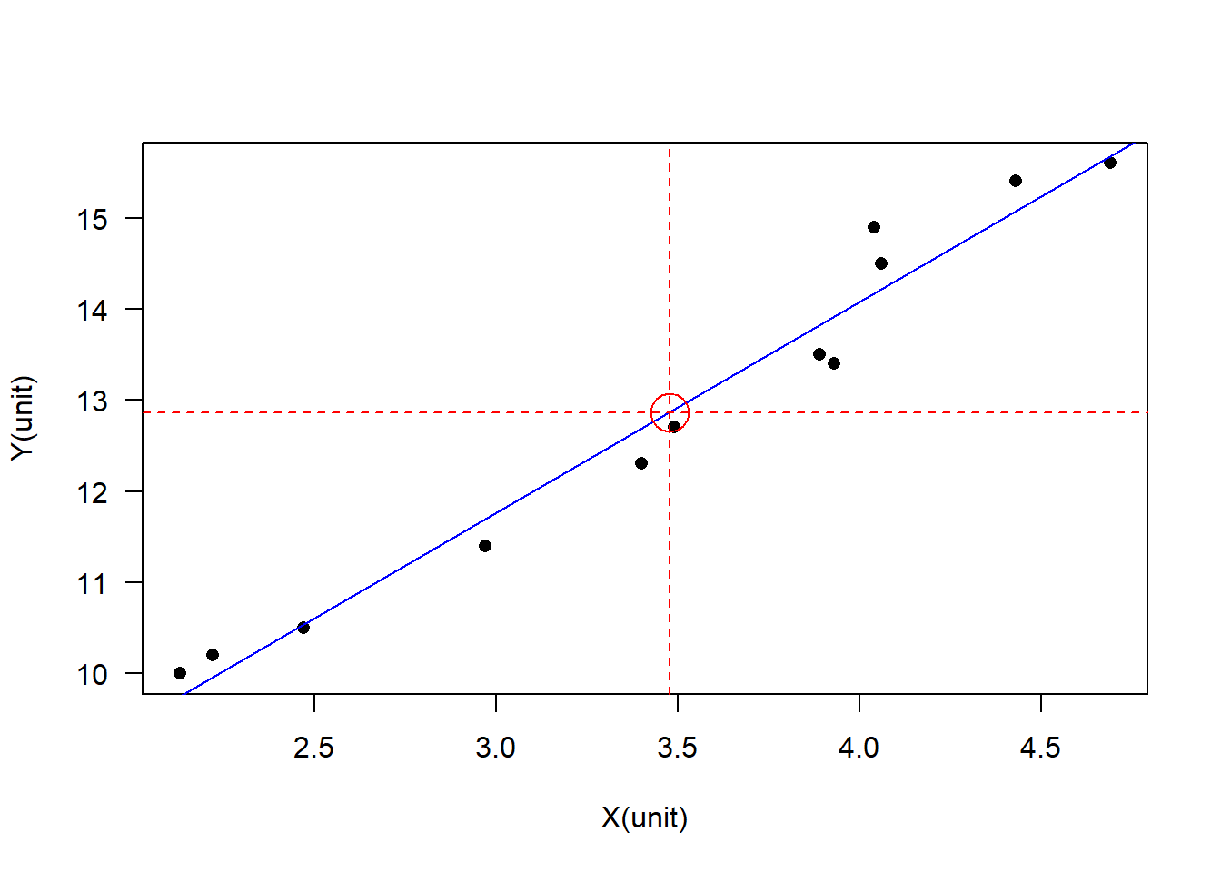

SessionInfo:

R version 4.2.3 (2023-03-15 ucrt)
Platform: x86_64-w64-mingw32/x64 (64-bit)
Running under: Windows 10 x64 (build 19044)

Matrix products: default

locale:
[1] LC_COLLATE=Chinese (Simplified)_China.utf8 
[2] LC_CTYPE=Chinese (Simplified)_China.utf8   
[3] LC_MONETARY=Chinese (Simplified)_China.utf8
[4] LC_NUMERIC=C                               
[5] LC_TIME=Chinese (Simplified)_China.utf8    

attached base packages:
[1] stats     graphics  grDevices utils     datasets  methods   base     

other attached packages:
[1] GGally_2.1.2  ggplot2_3.4.2

loaded via a namespace (and not attached):
 [1] Rcpp_1.0.10        plyr_1.8.8         RColorBrewer_1.1-3 pillar_1.9.0      
 [5] compiler_4.2.3     tools_4.2.3        digest_0.6.31      jsonlite_1.8.4    
 [9] evaluate_0.20      lifecycle_1.0.3    tibble_3.2.1       gtable_0.3.3      
[13] nlme_3.1-162       lattice_0.20-45    mgcv_1.8-42        pkgconfig_2.0.3   
[17] rlang_1.1.0        Matrix_1.5-3       cli_3.6.1          rstudioapi_0.14   
[21] yaml_2.3.7         xfun_0.37          fastmap_1.1.0      withr_2.5.0       
[25] dplyr_1.1.0        knitr_1.42         generics_0.1.3     vctrs_0.6.2       
[29] htmlwidgets_1.6.2  grid_4.2.3         tidyselect_1.2.0   reshape_0.8.9     
[33] glue_1.6.2         R6_2.5.1           fansi_1.0.3        rmarkdown_2.21    
[37] farver_2.1.1       magrittr_2.0.3     scales_1.2.1       htmltools_0.5.4   
[41] splines_4.2.3      colorspace_2.1-0   labeling_0.4.2     utf8_1.2.3        
[45] munsell_0.5.0